Graph Contrastive Learning

An explanation of node-level Graph Contrastive Learning

Graph neural networks have become very popular and often rely on learning representations for downstream tasks. This blog post will discuss graph contrastive learning, an unsupervised learning technique to construct representations from unlabelled data. The idea is based on slightly modifying the graphs so that the model can learn the notion of similarity. We will present the main ideas behind graph contrastive learning and reference the underlying literature. However, for a more thorough introduction, we recommend the reviews from Liu et al. and Xie et al., which cover the topic in-depth and have inspired this post.

Introduction

Although the amount of available data has steadily increased, much of it is neither processed nor annotated. While hand labeling might be an option for a relatively small number of samples, it is usually infeasible in real-world scenarios. Self-supervised learning is a way to make use of large amounts of unlabelled data to learn meaningful representations by exploiting the implicit structure. Representations are a compact way to describe the most important aspects of data in many different domains. For example, representations can capture the essence of words, proteins or represent the nodes of a graph. These representations can later be used as input to a neural network that predicts a label for each node, which only needs a few annotated samples for fine-tuning.

Self-supervised learning is most prominently used in computer vision tasks, such as image denoising, but also in natural language processing. Contrastive learning is a concrete method of self-supervised learning that learns representations so that similar structures in the data share similar representations.

Idea of (image) contrastive learning. The representation of different versions of the same images should agree with each other (blue), while they should be distinguishable from the other images (red).

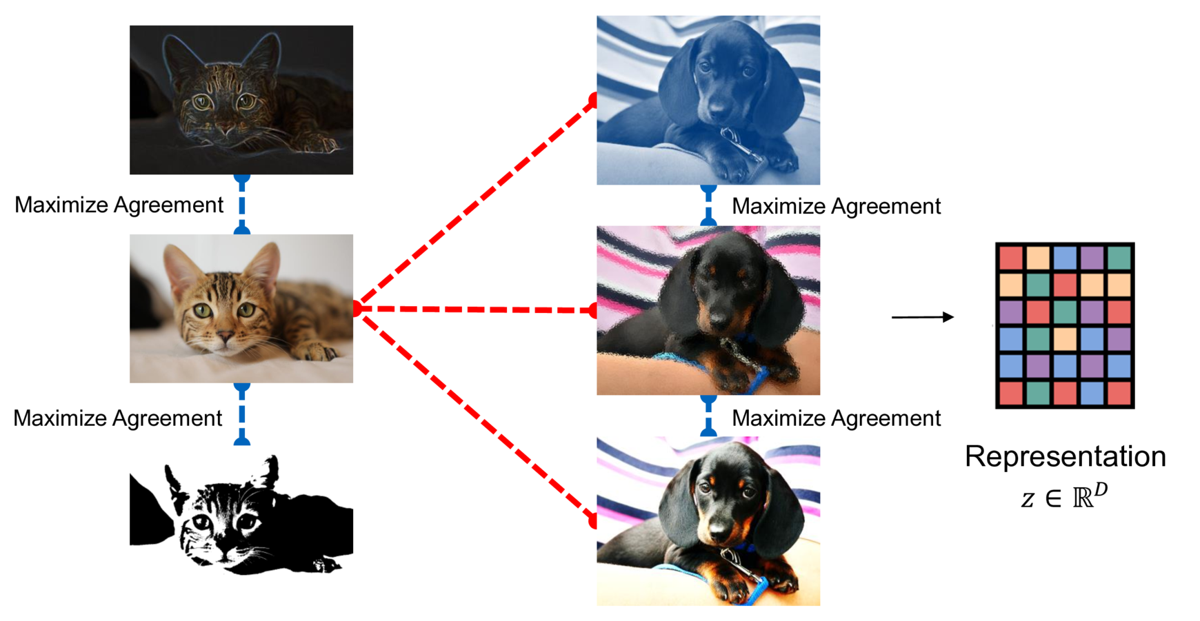
A simple example best explains the idea of contrastive learning. Consider pictures of cats and dogs, as seen in the figure above. We perform (minor) image augmentation techniques on the original pictures, such as changing the contrast or rotating and cropping the image. Although the pictures have been altered, the underlying semantic meaning does not change. All pictures of the cat are still pictures of the same cat, and all dog pictures still show the same dog. The idea behind contrastive learning is that augmentations of the same picture should have a similar representation. On the other hand, the difference in representation to all other images (such as pictures of dogs or other cats) should be as large as possible.

Although contrastive learning has originally been introduced for images, it can also be applied to different data types, such as graphs. Graphs have become a popular way of representing data in various fields. For example, molecular graphs are typically very large and lack labels making them ideal candidates for contrastive learning. Graph Contrastive Learning (GCL) is similar to image contrastive learning: the ultimate goal is to learn representations, but the representations of similar nodes should lie as close as possible in the latent spaceGraph Contrastive Learning can be defined on different levels to find embeddings for complete graphs or individual nodes. This blog post will focus on local-local contrasts where we compare nodes. See this awesome-list for papers sorted by different contrasting levels..

Pipeline of Graph Contrastive Learning. We create multiple views by augmenting an initial graph (left). The same nodes in different views (yellow) form positive pairs (blue), while all other nodes serve as contrasting pairs (red). An encoder (typically a neural network) and a projection head produce the representations.

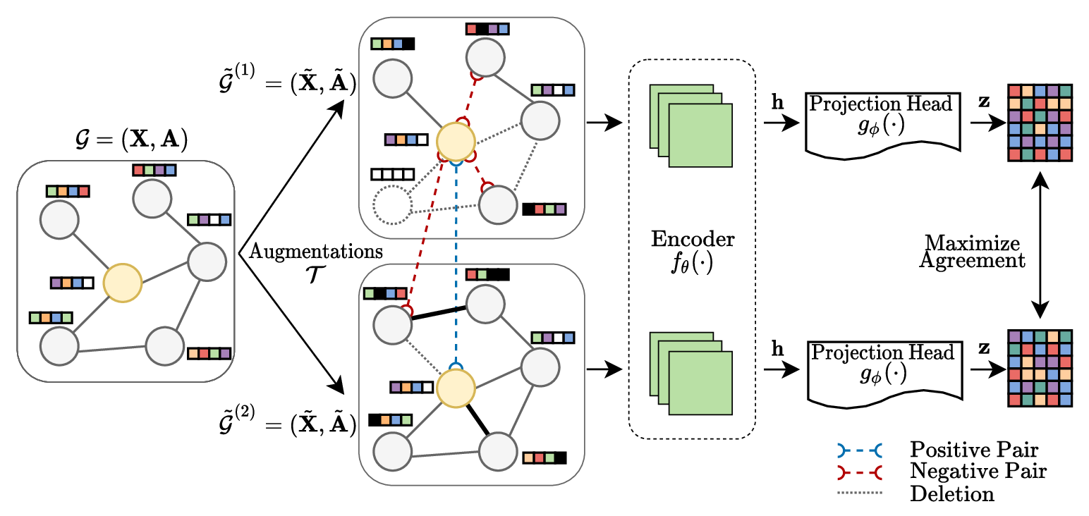
The figure above illustrates how GCL works and is the pipeline we will follow throughout this post. Instead of augmenting images, a graph is altered (edges or nodes deleted, features changed, etc.) to create different versions of the same graph. However, as with the images, the nodes should still have the same semantic meaning. A Graph Neural Network (encoder) then determines representations based on a loss that maximizes the agreement of similar nodes. This loss is defined so that the representation of the same nodes in different graph views should be pulled together. In the following, we will discuss these steps in more detail.

---

Graphs and Augmentations

Click here for the mathematical definition of graphs and their representations

We define a graph with \(N\) vertices as the core underlying object such that \(\mathcal{G} = (\mathbf X, \mathbf A)\). \(\mathbf{X} \in \mathbb{R}^{N \times F}\) denotes the feature matrix with \(F\) features and \(\mathbf A \in \mathbb{R}^{N \times N}\) is the adjacency matrix. While neural networks typically do not work well on this structure, Graph Neural Networks (GNNs) were introduced to overcome the problems.

Graphs are usually variable in size (i.e., the number of vertices and edges); hence, a fixed-size numeric representation can be valuable. Such representations are typically \(D\)-dimensional vectors in \(\mathbb{R}^{D}\), which compactly describe nodes or complete graphs.

In contrastive learning, the goal is to automatically find representations by leveraging a large amount of unlabeled data by generating contrastive views. In image contrastive learning, those views are created by augmentations that are usually straightforward. To name just a few, pictures can be cropped, rotated, or the contrast changed. However, graphs are structured fundamentally different than images, and operations that work on images, typically do not transfer to graphs. Depending on the data stored in the nodes or the edges of a graph, only a few augmentation techniques are applicable.

Graph augmentations form the basis of contrastive learning, as they provide the point of reference during: they determine which nodes are similar and thus, which representations need to be pulled together in the latent space. To formalize this, an augmentation function \(\mathcal{T}\) changes an original graph \(\mathcal G\) and creates different views \(\tilde{\mathcal G}\) by modifying the adjacency and feature matrix

\[\tilde{\mathcal G} = \mathcal{T}\left(\mathcal G) = (\mathcal{T}_{\mathbf{X}}(\mathbf X), \mathcal{T}_{\mathbf{A}}(\mathbf A)\right) \text{.}\]

1. Graph Topology Transformation

Modifying the underlying topology is the most straightforward and intuitive way to augment a graph. Changing the topology means we delete or add edges and vertices but do not change the data they store. A very primitive implementation of a topology-changing transformation would be to specify a ratio that determines how likely nodes or edges are removed. Many GCL algorithms rely on (simple) graph structure transformations. Graph diffusion is a more sophisticated approach that uses a random walk and thus, information from a larger neighborhood to decide which nodes or edges to keep. In the end, all those approaches mainly change the adjacency matrix \(\mathbf A\).

2. Node Feature Transformation

The second major way to agument a graph are feature-modifying augmentations which modify the feature matrix \(\mathbf X\) and with it the actual data stored. A very common and straightforward technique to augment the features is node feature masking, where values of the feature matrix \(\mathbf X\) are randomly replaced with a different value (typically zero). Another widely used technique is node feature shuffling, where features of nodes are randomly swapped.

Depending on the concrete data stored for every node, adapting the features has drastically different capabilities. For example, consider a graph where every node stores an image. In such a setting, classical contrastive learning techniques, where images are rotated or the color space changed, are possible and likely lead to better results than primitive feature transformations.

3. Other Methods

Combining augmentations that change the topology and features is better than relying on only one of those types. So-called hybrid methods combine multiple augmentation techniques and are widely used. For example, one can drop edges and mask features simultaneously or combine even more different approaches. Instead of deleting elements, there also exists subgraph sampling, where only a specific portion of the graph is randomly selected and used. In its simplest form, nodes, and edges are uniformly sampled from the original graph, but again there are approaches based on random walks that allow us to explore the neighborhood more selectively.

Augmentations in graphs need to be hand-picked and fine-tuned. For every graph, different augmentations work better. Adaptive augmentations make this process easier by detecting and retaining the essential features while applying more noise in less critical parts. You et al., on the other hand, propose an approach that automates augmentations altogether. They introduce a bi-level optimization technique where the augmentation resulting in the highest loss is selected in each training step. When combining this with a different projection head for each augmentation, their method can outperform existing algorithms.

4. Augmentation “Free” Methods

Some methods eliminate the need for augmentations altogether, such as graph soft-contrastive learning, which relies on the homophilicity of graphs. In homophilic graphs, the number of hops between two nodes determines their similarity. Research graphs, for example, are typically homophilic, as papers that cite each other are usually similar. The authors of soft-contrastive learning argue that classical augmentation techniques have issues with homophilic graphs since close neighbors are already seen as contrasting pairs. They change the loss in such a way that the distance between the nodes determines the similary. This leads to better representations in homophilic graphs.

Similarly, Wang et al. argue that augmentations are also flawed in the opposite case when neighbors are not similar. They introduce an algorithm that aggregates node features and optimizes the representation space directly to solve this issue.

---

Learning Representations

In the previous section, we discussed how to construct contrastive views with various augmentation techniques. With this wide range of different ways to generate contrasting views we can discuss how to learn representations. In the following, we will continue with the remaining parts of the pipeline: the actual models and how to train them. Now is a good time to look at the pipeline of GCL from before again to put this into context.

The Encoder and Projection Heads

The encoder \(f_\theta : \mathcal{G} \to \mathbb{R}^{N \times D}\) is the core part of the contrastive model and generates a representation \(\mathbf{h}_i\) for each node in the graph \(\mathcal{G}\). In principle, any model can be used to calculate the representations, but usually, graph neural networks (GNNs) are used as they have shown to work especially well int this context.

In addition to the encoder, Chen et al. advocate for the introduction of so-called projection heads: functions \(g_\phi : \mathbb{R}^{D} \to \mathbb{R}^{K}\) that map a representation \(\mathbf{h}_i\) again to produce a more sophisticated representation \(\textbf{z}_i = g_\phi (\mathbf{h}_i)\). With them, the model can undo the augmentations and learn the same representation for different augmentations. Typically, projection heads are small multi-layer perceptrons with either two or three layers. Some architectures do not include any at all. Non-linear projection heads can greatly increase the performance of (image) contrastive learning because they introduce additional flexibility.

During training, the projection head and the encoder, determine the representations \(\textbf{z} = g_\phi \circ f_\theta \left( \mathcal{G} \right)\) of all nodes in a graph. At inference, often only the encoder is used to create representation. This is because at inference, there is no need to “unlearn the augmentations”, because there will not be any applied.

Optimization

The encoder and projection heads need to be trained with a suitable loss to achieve the property that similar nodes have similar representations. While there are many possibilities to define the optimization target, we will focus on a minimization that only uses two augmented graph views produced by a single graph. This setting has been shown to yield good empirical results. The general optimization target to determine the optimal parameters is

\[\theta^*, \phi^* = \underset{\theta, \phi}{\arg \min}~ \mathcal{L}_{con} \left(g_\phi\left(f_\theta\left(\tilde{\mathcal{G}}^{(1)}\right)_i~\right), g_\phi\left(f_\theta\left(\tilde{\mathcal{G}}^{(2)}\right)_j\right)\right) \text{,}\]

where \(\mathcal{L}_{con}\) is a contrastive loss that takes the representations of two similar nodes (i.e., a positive pairs) \(i\) and \(j\) in two different views \(\tilde{\mathcal{G}}^{(1)}\) and \(\tilde{\mathcal{G}}^{(2)}\) respectively. The goal of any contrastive loss \(\mathcal{L}_{con}\) is to pull representations of positive pairs close to each other while pushing negative pairs apart. In practice, there are many different concrete contrastive losses to choose from.

Mutual Information

Approximating the mutual information is the basis for most contrastive learning losses. Mutual information describes the information that is shared by two random variables and is defined as

\[\begin{aligned} \mathcal{M}\mathcal{I}(\boldsymbol{x}, \boldsymbol{y}) &= D_{K L}(p(\boldsymbol{x}, \boldsymbol{y})~\|~p(\boldsymbol{x}) p(\boldsymbol{y})) \\ &=\mathbb{E}_{p(\boldsymbol{x}, \boldsymbol{y})}\left[\log \frac{p(\boldsymbol{x}, \boldsymbol{y})}{p(\boldsymbol{x}) p(\boldsymbol{y})}\right] \text{.} \end{aligned}\]

\(D_{K L}\) is the Kullback–Leibler divergence and is a difference between two distributions. In this case, the joint probability \(p(\boldsymbol{x}, \boldsymbol{y})\) describes the shared amount of information, while the multiplication of marginal densities \(p(\boldsymbol{x}) p(\boldsymbol{y})\) describes their dissimilarity.

While mutual information forms the basis of most contrastive losses, calculating the exact value is notoriously difficult and hence, estimates of it are used in practice. In the following paragraphs, we will focus on two of such estimates of mutual information to train the encoder \(f_\theta\) and the projection head \(g_\phi\).

Jensen-Shannon Estimator

The Jensen-Shannon Divergence (JSD) can be used as an approximation for the mutual information. It is one of the most commonly used lower bounds for graph contrastive learning and is especially suitable for cases where the downstream task is to classify graphs based on node representations. Following the definition from Liu et al., the Jensen-Shannon estimator can be written as

\[\begin{aligned} \mathcal{L}_{\text {con }}\left(\mathbf{z}_i, \mathbf{z}_j\right)&=-\mathcal{M} \mathcal{I}_{J S D}\left(\mathbf{z}_i, \mathbf{z}_j\right) \\ &= \mathbb{E}_{\left( \mathbf{z}_i, \mathbf{z}_j^{\prime}\right)}\left[\log \left(1-s\left(\mathbf{z}_i, \mathbf{z}_j^{\prime}\right)\right)\right] - \log \left(s\left(\mathbf{z}_i, \mathbf{z}_j\right)\right) \text{.} \end{aligned}\]

\(s( \cdot, \cdot )\) is a similarity function and is typically the cosine similarity of the representations, or the dot productWhen one uses the sigmoid function after the similarity function is applied, the JSD loss forms the basis for the widely known InfoGraph architecture.. Using a more complex function is not necessary since projection heads can learn a different latent space.

The contrastive loss is computed for all similar pairs of nodes \(\left(\mathbf{z}_i, \mathbf{z}_j\right)\). For JSD, the similarity of this positive pair is then compared to all other negative pairs \(\left(\mathbf{z}_i, \mathbf{z}_j^{\prime}\right)\) sharing the node \(i\). This gives us the relative strength of this positive connection, similarly to as is done in the mutual information. We can also see that there is an expected value here, meaning that we would have to integrate over all negative pairs, which is usually difficult to calculate. In practice, the expected value is approximated as an average over all available negative pairs in the current views. For this, we can use negative pairs of nodes in the same graph or between nodes in different views.

Noise-Contrastive Estimator

Another widely used estimator is the noise-contrastive estimator which is more typically referred to as InfoNCE. In this case, the loss is defined as

\[\begin{aligned} \mathcal{L}_{\text {con }}\left(\mathbf{z}_i, \mathbf{z}_j\right)&=-\mathcal{M} \mathcal{I}_{N C E}\left(\mathbf{z}_i, \mathbf{z}_j\right) \\ &=-\log \frac{e^{s\left(\mathbf{z}_i, \mathbf{z}_j\right)}}{e^{s\left(\mathbf{z}_i, \mathbf{z}_j\right)}+\sum_{\mathbf{z}_j^{\prime}} e^{s\left(\mathbf{z}_i, \mathbf{z}_j^{\prime}\right)}} ~ \text{,} \end{aligned}\]

where \(\left(\mathbf{z}_i, \mathbf{z}_j\right)\) is again a positive pair, \(\mathbf{z}_j^{\prime}\) are negative pairs for the representation of node \(i\), and \(s( \cdot, \cdot)\) a similarity function. Pairs that are similar according to \(s( \cdot, \cdot)\) will then have a representation close in the latent space. Similarly to the Jensen-Shannon estimator, InfoNCE maximizes the relative similarity of positive pairs compared to their respective negative pairs. In many cases InfoNCE can outperform Jensen-Shannon estimator, but this effect diminishes with larger datasets.

There is a variety of additional different losses available for graph contrastive learning such as Donsker-Varadhan objective which is equivalent to InfoNCE, the triplet margin loss which is similar to InfoNCE but does not provide mathematical guarantees when it is used for graph contrastive learning. Furthermore, there is also the BYOL loss or the Barlow Twins Loss. Hassani et al. compare various losses in their work and examine their effects on training.

---

Discussion

Graph contrastive learning is a technique to learn representations in a self-supervised setting by exploiting the graph’s structure with augmentations to create contrastive views. Most work in the field is a direct extension of the image domain, and typically only empirical results are available. Extending algorithms to graphs is challenging, and there are still some open issues. For example, the usefulness of projection heads has only been examined in image contrastive learning by Chen et al., and the idea was transferred to graphs. Graph-specific projection heads, or even projection head-free methods, might be more suitable and may lead to improved results.

As of writing, choosing the correct graph augmentations is difficult because they typically rely on (implicit) assumptions, such as homophily, which not every graph fulfills. A solid mathematical background or the question “What is the best augmentation function for my graph?” remains an open field of research. Most work in GCL relies on evaluating different augmentations on various datasets and empirically drawing conclusions from this. There is some research on augmentation-free methods which seems promising, and there are also ideas to find suitable augmentations automatically. Researching more robust augmentations or procedures capable of learning augmentations could benefit the community. There are similar techniques that do not rely on negative samples. In invariant regularization for example, the goal is to make representations of augmented views as similar as possible instead of contrasting positive and negative pairs.

Although GCL has its issues and the performance varies drastically between use cases, it is still promising and can benefit many areas. Especially using GCL as a pre-training step is an easy way to use unlabeled data.

---

Acknowledgements

Thank you Filippo Guerranti for our fruitful discussions and your help in revising this document.